Simple ion plan optimization and DICOM study creation

author: OpenTPS team

In this example, we will create and optimize a simple ion (Proton) plan. The generated CT, the plan, and the dose will be saved as DICOM files.

running time: ~ 15 minutes

Setting up the environment in google collab

import sys
if "google.colab" in sys.modules:
    from IPython import get_ipython
    get_ipython().system('git clone https://gitlab.com/openmcsquare/opentps.git')
    get_ipython().system('pip install ./opentps')

    import opentps

imports

import os
import logging
import numpy as np
from matplotlib import pyplot as plt
import sys
import datetime
import pydicom
sys.path.append('..')

import the needed opentps.core packages

import opentps.core.processing.planOptimization.objectives.dosimetricObjectives as doseObj
from opentps.core.io.dicomIO import writeRTPlan, writeDicomCT, writeRTDose, writeRTStruct
from opentps.core.processing.planOptimization.tools import evaluateClinical
from opentps.core.data.images import CTImage, DoseImage
from opentps.core.data.images import ROIMask
from opentps.core.data.plan import ObjectivesList
from opentps.core.data.plan._protonPlanDesign import ProtonPlanDesign
from opentps.core.data import DVH
from opentps.core.data import Patient
from opentps.core.data import RTStruct
from opentps.core.io import mcsquareIO
from opentps.core.io.scannerReader import readScanner
from opentps.core.io.serializedObjectIO import saveRTPlan, loadRTPlan
from opentps.core.processing.doseCalculation.doseCalculationConfig import DoseCalculationConfig
from opentps.core.processing.doseCalculation.protons.mcsquareDoseCalculator import MCsquareDoseCalculator
from opentps.core.processing.imageProcessing.resampler3D import resampleImage3DOnImage3D, resampleImage3D
from opentps.core.processing.planOptimization.planOptimization import IntensityModulationOptimizer
from opentps.core.data.plan import ProtonPlan

logger = logging.getLogger(__name__)

CT calibration and BDL

ctCalibration = readScanner(DoseCalculationConfig().scannerFolder)
bdl = mcsquareIO.readBDL(DoseCalculationConfig().bdlFile)

Create the DICOM files

 # ++++Don't delete UIDs to build the simple study+++++++++++++++++++
studyInstanceUID = pydicom.uid.generate_uid()
doseSeriesInstanceUID = pydicom.uid.generate_uid()
planSeriesInstanceUID = pydicom.uid.generate_uid()
ctSeriesInstanceUID =  pydicom.uid.generate_uid()
frameOfReferenceUID = pydicom.uid.generate_uid()
# structSeriesInstanceUID = pydicom.uid.generate_uid()
dt = datetime.datetime.now()
#++++++++++++++++++++++++++++++++++++++++++++++++++++++++++++++++

Output path

output_path = 'Output'
if not os.path.exists(output_path):
    os.makedirs(output_path)

Generic CT creation

we will first create a generic CT of a box fill with water and air

patient = Patient()
patient.name = 'Simple_Patient'
Patient.id = 'Simple_Patient'
Patient.birthDate = dt.strftime('%Y%m%d')
patient.sex = ""

ctSize = 150
ct = CTImage(seriesInstanceUID=ctSeriesInstanceUID, frameOfReferenceUID=frameOfReferenceUID)
ct.name = 'CT'
ct.patient = patient
ct.studyInstanceUID = studyInstanceUID

huAir = -1024.
huWater = ctCalibration.convertRSP2HU(1.)
data = huAir * np.ones((ctSize, ctSize, ctSize))
data[:, 50:, :] = huWater
ct.imageArray = data
writeDicomCT(ct, output_path)

/opt/hostedtoolcache/Python/3.12.12/x64/lib/python3.12/site-packages/pydicom/valuerep.py:440: UserWarning: A value of type 'int64' cannot be assigned to a tag with VR US.
  warn_and_log(msg)

'1.2.826.0.1.3680043.8.498.97208472055841171788042654448685095284'

Region of interest

we will now create a region of interest wich is a small 3D box of size 20*20*20

roi = ROIMask()
roi.patient = patient
roi.name = 'TV'
roi.color = (255, 0, 0)  # red
data = np.zeros((ctSize, ctSize, ctSize)).astype(bool)
data[100:120, 100:120, 100:120] = True
roi.imageArray = data

body = roi.copy()
body.name = 'Body'
body.dilateMask(20)
body.imageArray = np.logical_xor(body.imageArray, roi.imageArray).astype(bool)

Configuration of Mcsquare

To configure the MCsquare calculator we need to calibrate it with the CT calibration obtained above

mc2 = MCsquareDoseCalculator()
mc2.beamModel = bdl
mc2.nbPrimaries = 5e4
mc2.ctCalibration = ctCalibration

Plan Creation

 # Design plan
beamNames = ["Beam1"]
gantryAngles = [0.]
couchAngles = [0.]

# Load / Generate new plan
plan_file = os.path.join(output_path, "Plan_WaterPhantom_cropped_resampled.tps")

if os.path.isfile(plan_file):
    plan = loadRTPlan(plan_file)
    logger.info('Plan loaded')
else:
    planDesign = ProtonPlanDesign()
    planDesign.ct = ct
    planDesign.targetMask = roi
    planDesign.gantryAngles = gantryAngles
    planDesign.beamNames = beamNames
    planDesign.couchAngles = couchAngles
    planDesign.calibration = ctCalibration
    planDesign.spotSpacing = 5.0
    planDesign.layerSpacing = 5.0
    planDesign.targetMargin = 5.0
    planDesign.setScoringParameters(scoringSpacing=[2, 2, 2], adapt_gridSize_to_new_spacing=True)
    planDesign.defineTargetMaskAndPrescription(target = roi, targetPrescription = 20.) # needs to be called prior spot placement

    plan = planDesign.buildPlan()  # Spot placement
    plan.rtPlanName = "Simple_Patient"

    beamlets = mc2.computeBeamlets(ct, plan, roi=[roi,body])
    plan.planDesign.beamlets = beamlets
    beamlets.storeOnFS(os.path.join(output_path, "BeamletMatrix_" + plan.seriesInstanceUID + ".blm"))
    # Save plan with initial spot weights in serialized format (OpenTPS format)
    saveRTPlan(plan, plan_file)
    writeRTPlan(plan, output_path)

objectives

# Set objectives (attribut is already initialized in planDesign object)
plan.planDesign.objectives.addObjective(doseObj.DMax(body,5, weight=1.0))

plan.planDesign.objectives.addObjective(doseObj.DMax(roi, 21, weight=10.0))
plan.planDesign.objectives.addObjective(doseObj.DMin(roi, 20, weight=20.0))

Optimize plan

plan.seriesInstanceUID = planSeriesInstanceUID
plan.studyInstanceUID = studyInstanceUID
plan.frameOfReferenceUID = frameOfReferenceUID
plan.rtPlanGeometry = "TREATMENT_DEVICE"

solver = IntensityModulationOptimizer(method='Scipy_L-BFGS-B', plan=plan, maxiter=1000)
# Optimize treatment plan
doseImage, ps = solver.optimize()

# Save plan with updated spot weights in serialized format (OpenTPS format)
plan_file_optimized = os.path.join(output_path, "Plan_WaterPhantom_cropped_resampled_optimized.tps")
saveRTPlan(plan, plan_file_optimized)
# Save plan with updated spot weights in dicom format
plan.patient = patient
writeRTPlan(plan, output_path)

/opt/hostedtoolcache/Python/3.12.12/x64/lib/python3.12/site-packages/pydicom/valuerep.py:440: UserWarning: Invalid value for VR CS: 'RT Ion Plan IOD'. Please see <https://dicom.nema.org/medical/dicom/current/output/html/part05.html#table_6.2-1> for allowed values for each VR.
  warn_and_log(msg)
/opt/hostedtoolcache/Python/3.12.12/x64/lib/python3.12/site-packages/pydicom/dataset.py:2710: UserWarning: Camel case attribute 'PrivateCreator' used which is not in the element keyword data dictionary
  warn_and_log(msg)

Dose volume histogram

target_DVH = DVH(roi, doseImage)
body_DVH = DVH(body, doseImage)
print('D5 - D95 =  {} Gy'.format(target_DVH.D5 - target_DVH.D95))
clinROI = [roi.name, roi.name]
clinMetric = ["Dmin", "Dmax"]
clinLimit = [19., 21.]
clinObj = {'ROI': clinROI, 'Metric': clinMetric, 'Limit': clinLimit}
print('Clinical evaluation')
evaluateClinical(doseImage, [roi], clinObj)

doseImage.referencePlan = plan
doseImage.referenceCT = ct
doseImage.patient = patient
doseImage.studyInstanceUID = studyInstanceUID
doseImage.frameOfReferenceUID = frameOfReferenceUID
doseImage.sopClassUID = '1.2.840.10008.5.1.4.1.1.481.2'
doseImage.mediaStorageSOPClassUID = '1.2.840.10008.5.1.4.1.1.481.2'
doseImage.sopInstanceUID = pydicom.uid.generate_uid()
doseImage.studyTime = dt.strftime('%H%M%S.%f')
doseImage.studyDate = dt.strftime('%Y%m%d')
doseImage.SOPInstanceUID = doseImage.sopInstanceUID

if not hasattr(ProtonPlan, "SOPInstanceUID"):
    ProtonPlan.SOPInstanceUID = property(lambda self: self.sopInstanceUID)


writeRTDose(doseImage, output_path)

D5 - D95 =  3.5624186197916643 Gy
Clinical evaluation
----------------------------------------------------------------------------------------------------
ROI            Metric    Limit   D98/D2   Passed D95/D5   Passed
----------------------------------------------------------------------------------------------------
TV             Dmin      19.00   18.51      0    18.80      0
TV             Dmax      21.00   22.57      0    22.37      0
/opt/hostedtoolcache/Python/3.12.12/x64/lib/python3.12/site-packages/pydicom/dataset.py:2710: UserWarning: Camel case attribute 'SoftwareVersion' used which is not in the element keyword data dictionary
  warn_and_log(msg)
/opt/hostedtoolcache/Python/3.12.12/x64/lib/python3.12/site-packages/pydicom/dataset.py:2710: UserWarning: Camel case attribute 'OperatorName' used which is not in the element keyword data dictionary
  warn_and_log(msg)
/opt/hostedtoolcache/Python/3.12.12/x64/lib/python3.12/site-packages/pydicom/dataset.py:2710: UserWarning: Camel case attribute 'Width' used which is not in the element keyword data dictionary
  warn_and_log(msg)
/opt/hostedtoolcache/Python/3.12.12/x64/lib/python3.12/site-packages/pydicom/dataset.py:2710: UserWarning: Camel case attribute 'Height' used which is not in the element keyword data dictionary
  warn_and_log(msg)
/opt/hostedtoolcache/Python/3.12.12/x64/lib/python3.12/site-packages/pydicom/dataset.py:2710: UserWarning: Camel case attribute 'ColorType' used which is not in the element keyword data dictionary
  warn_and_log(msg)
/opt/hostedtoolcache/Python/3.12.12/x64/lib/python3.12/site-packages/pydicom/dataset.py:2710: UserWarning: Camel case attribute 'BitDepth' used which is not in the element keyword data dictionary
  warn_and_log(msg)

Center of mass

Here we look at the part of the 3D CT image where “stuff is happening” by getting the CoM. We use the function resampleImage3DOnImage3D to the same array size for both images.

roi = resampleImage3DOnImage3D(roi, ct)
COM_coord = roi.centerOfMass
COM_index = roi.getVoxelIndexFromPosition(COM_coord)
Z_coord = COM_index[2]

img_ct = ct.imageArray[:, :, Z_coord].transpose(1, 0)
img_mask = roi.imageArray[:, :, Z_coord].transpose(1, 0)
img_body = body.imageArray[:, :, Z_coord].transpose(1, 0)
img_dose = resampleImage3DOnImage3D(doseImage, ct)
img_dose = img_dose.imageArray[:, :, Z_coord].transpose(1, 0)

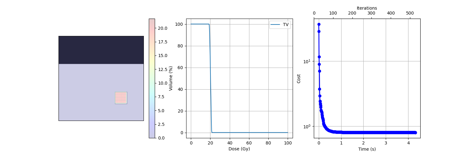
Plot of the dose

fig, ax = plt.subplots(1, 3, figsize=(15, 5))
ax[0].axes.get_xaxis().set_visible(False)
ax[0].axes.get_yaxis().set_visible(False)
ax[0].imshow(img_ct, cmap='gray')
ax[0].contour(img_body,[0.5],colors='green')  # Body
ax[0].contour(img_mask,[0.5],colors='red')
dose = ax[0].imshow(img_dose, cmap='jet', alpha=.2)
plt.colorbar(dose, ax=ax[0])
ax[1].plot(target_DVH.histogram[0], target_DVH.histogram[1], label=target_DVH.name,color='red')
ax[1].plot(body_DVH.histogram[0], body_DVH.histogram[1], label=body_DVH.name,color='green')
ax[1].set_xlabel("Dose (Gy)")
ax[1].set_ylabel("Volume (%)")
ax[1].grid(True)
ax[1].legend()

convData = solver.getConvergenceData()
ax[2].plot(np.linspace(0, convData['time'], len(convData['func_0'])), convData['func_0'], 'bo-', lw=2,
            label='Fidelity')
ax[2].set_xlabel('Time (s)')
ax[2].set_ylabel('Cost')
ax[2].set_yscale('symlog')
ax2 = ax[2].twiny()
ax2.set_xlabel('Iterations')
ax2.set_xlim(0, convData['nIter'])
ax[2].grid(True)

plt.savefig(f'{output_path}/Dose_SimpleOptimization.png', format = 'png')
plt.show()