Beamlet Free Optimization

author: OpenTPS team

This example will present the basis of beamlet optimization with openTPS core.

running time: ~ 15 minutes

Setting up the environment in google collab

import sys
if "google.colab" in sys.modules:
    from IPython import get_ipython
    get_ipython().system('git clone https://gitlab.com/openmcsquare/opentps.git')
    get_ipython().system('pip install ./opentps')
    get_ipython().system('pip install scipy==1.10.1')
    import opentps

imports

import numpy as np
import os
from matplotlib import pyplot as plt

import the needed opentps.core packages

from opentps.core.data.images import CTImage
from opentps.core.data.images import ROIMask
from opentps.core.data.plan import ObjectivesList
from opentps.core.data.plan._protonPlanDesign import ProtonPlanDesign
from opentps.core.data import DVH
from opentps.core.data import Patient
from opentps.core.data.plan import FidObjective
from opentps.core.io import mcsquareIO
from opentps.core.io.scannerReader import readScanner
from opentps.core.processing.doseCalculation.doseCalculationConfig import DoseCalculationConfig
from opentps.core.processing.doseCalculation.protons.mcsquareDoseCalculator import MCsquareDoseCalculator
from opentps.core.processing.imageProcessing.resampler3D import resampleImage3DOnImage3D

Output path

output_path = 'Output'
if not os.path.exists(output_path):
    os.makedirs(output_path)

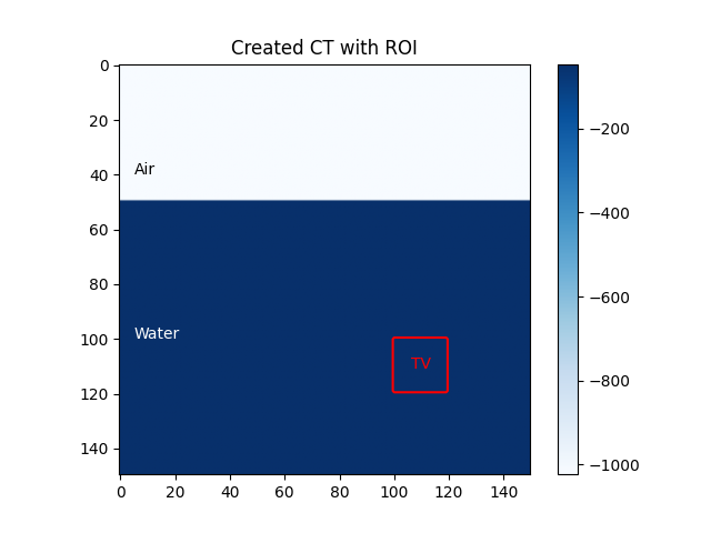
Generic CT creation

we will first create a generic CT of a box fill with water and air

#calibratioin of the CT
ctCalibration = readScanner(DoseCalculationConfig().scannerFolder)
bdl = mcsquareIO.readBDL(DoseCalculationConfig().bdlFile)

#creation of the patient object
patient = Patient()
patient.name = 'Patient'

#size of the 3D box
ctSize = 150

#creation of the CTImage object
ct = CTImage()
ct.name = 'CT'
ct.patient = patient

huAir = -1024. #Hounsfield unit of water
huWater = ctCalibration.convertRSP2HU(1.) #convert a stopping power of 1. to HU units
data = huAir * np.ones((ctSize, ctSize, ctSize))
data[:, 50:, :] = huWater
ct.imageArray = data #the CT generic image is created

Region of interest

we will now create a region of interest which is a small 3D box of size 20*20*20

roi = ROIMask()
roi.patient = patient
roi.name = 'TV'
roi.color = (255, 0, 0) # red
data = np.zeros((ctSize, ctSize, ctSize)).astype(bool)
data[100:120, 100:120, 100:120] = True
roi.imageArray = data

image = plt.imshow(ct.imageArray[110,:,:],cmap='Blues')
plt.colorbar(image)
plt.contour(roi.imageArray[110,:,:],colors="red")
plt.title("Created CT with ROI")
plt.text(5,40,"Air",color= 'black')
plt.text(5,100,"Water",color = 'white')
plt.text(106,111,"TV",color ='red')
plt.savefig(os.path.join(output_path,'beamFree1.png'),format = 'png')
plt.show()

Configuration of Mcsquare

To configure the MCsquare calculator we need to calibrate it with the CT calibration obtained above

mc2 = MCsquareDoseCalculator()
mc2.beamModel = bdl
mc2.ctCalibration = ctCalibration
mc2.nbPrimaries = 1e7

Plan Creation

We will now create a plan and set objectives for the optimization and set a goal of 20Gy to the target

# Design plan

beamNames = ["Beam1"]
gantryAngles = [0.]
couchAngles = [0.]

# Generate new plan

planDesign = ProtonPlanDesign() #create a new plan
planDesign.ct = ct
planDesign.gantryAngles = gantryAngles
planDesign.beamNames = beamNames
planDesign.couchAngles = couchAngles
planDesign.calibration = ctCalibration
planDesign.spotSpacing = 5.0
planDesign.layerSpacing = 5.0
planDesign.targetMargin = 5.0
# needs to be called prior to spot placement
planDesign.defineTargetMaskAndPrescription(target = roi, targetPrescription = 20.)


plan = planDesign.buildPlan()  # Spot placement
plan.PlanName = "NewPlan"

plan.planDesign.objectives.addFidObjective(roi, FidObjective.Metrics.DMAX, 20.0, 1.0)
plan.planDesign.objectives.addFidObjective(roi, FidObjective.Metrics.DMIN, 20.0, 1.0)

Mcsquare beamlet free planOptimization

Now that we have every needed objects we can compute the optimization through MCsquare. :warning: It may take some time to compute.

doseImage = mc2.optimizeBeamletFree(ct, plan, [roi])

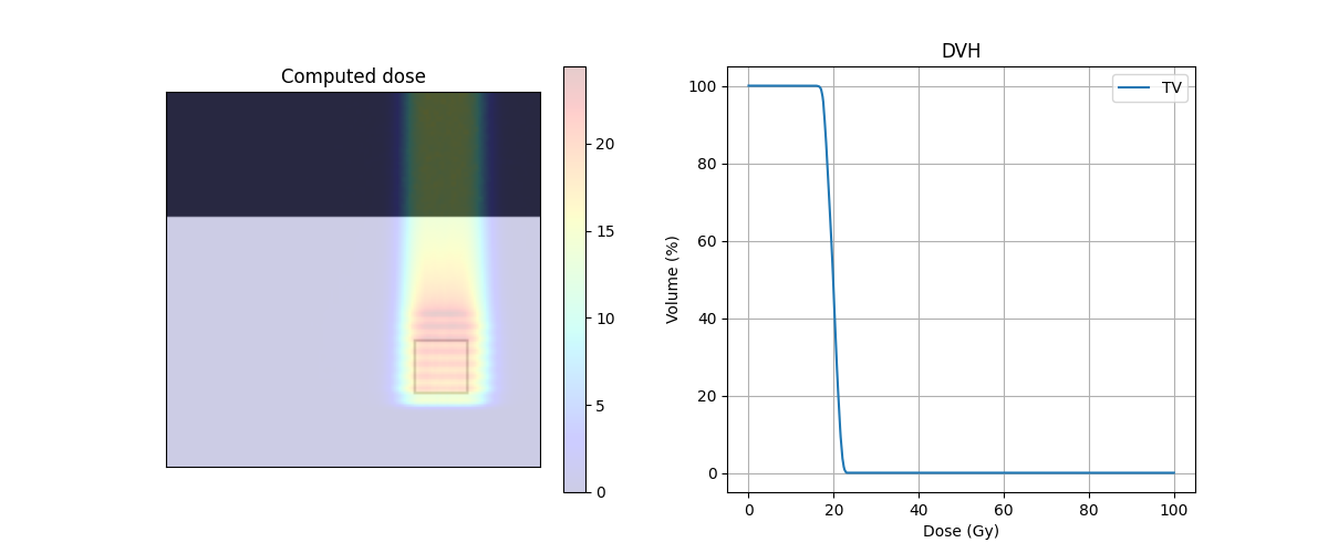
Dose volume histogram

target_DVH = DVH(roi, doseImage)
print('D95 = ' + str(target_DVH.D95) + ' Gy')
print('D5 = ' + str(target_DVH.D5) + ' Gy')
print('D5 - D95 =  {} Gy'.format(target_DVH.D5 - target_DVH.D95))

D95 = 17.60765281883446 Gy
D5 = 21.945953369140625 Gy
D5 - D95 =  4.338300550306165 Gy

Center of mass

Here we look at the part of the 3D CT image where “stuff is happening” by getting the CoM. We use the function resampleImage3DOnImage3D to the same array size for both images.

roi = resampleImage3DOnImage3D(roi, ct)
COM_coord = roi.centerOfMass
COM_index = roi.getVoxelIndexFromPosition(COM_coord)
Z_coord = COM_index[2]

img_ct = ct.imageArray[:, :, Z_coord].transpose(1, 0)
contourTargetMask = roi.getBinaryContourMask()
img_mask = contourTargetMask.imageArray[:, :, Z_coord].transpose(1, 0)
img_dose = resampleImage3DOnImage3D(doseImage, ct)
img_dose = img_dose.imageArray[:, :, Z_coord].transpose(1, 0)

Plot of the dose

fig, ax = plt.subplots(1, 2, figsize=(12, 5))
ax[0].axes.get_xaxis().set_visible(False)
ax[0].axes.get_yaxis().set_visible(False)
ax[0].imshow(img_ct, cmap='gray')
ax[0].imshow(img_mask, alpha=.2, cmap='binary')  # PTV
dose = ax[0].imshow(img_dose, cmap='jet', alpha=.2)
plt.colorbar(dose, ax=ax[0])
ax[1].plot(target_DVH.histogram[0], target_DVH.histogram[1], label=target_DVH.name)
ax[1].set_xlabel("Dose (Gy)")
ax[1].set_ylabel("Volume (%)")
ax[0].set_title("Computed dose")
ax[1].set_title("DVH")
plt.grid(True)
plt.legend()
plt.savefig(os.path.join(output_path,'beamFree2.png'),format = 'png')
plt.show()