Simple IMPT proton plan optimization

author: OpenTPS team

In this example, we will create and optimize a simple Protons plan.

running time: ~ 12 minutes

Setting up the environment in google collab

import sys
if "google.colab" in sys.modules:
    from IPython import get_ipython
    get_ipython().system('git clone https://gitlab.com/openmcsquare/opentps.git')
    get_ipython().system('pip install ./opentps')

    import opentps

imports

import math
import os
import sys

import numpy as np
from matplotlib import pyplot as plt

import the needed opentps.core packages

import opentps.core.processing.planOptimization.objectives.dosimetricObjectives as doseObj
from opentps.core.data.images import CTImage
from opentps.core.data.images import ROIMask
from opentps.core.data.plan import ObjectivesList
from opentps.core.data.plan import ProtonPlanDesign
from opentps.core.data import DVH
from opentps.core.data import Patient
from opentps.core.io import mcsquareIO
from opentps.core.io.scannerReader import readScanner
from opentps.core.io.serializedObjectIO import saveRTPlan, loadRTPlan
from opentps.core.processing.doseCalculation.doseCalculationConfig import DoseCalculationConfig
from opentps.core.processing.doseCalculation.protons.mcsquareDoseCalculator import MCsquareDoseCalculator
from opentps.core.processing.imageProcessing.resampler3D import resampleImage3DOnImage3D, resampleImage3D
from opentps.core.processing.planOptimization.planOptimization import IntensityModulationOptimizer

CT calibration and BDL

ctCalibration = readScanner(DoseCalculationConfig().scannerFolder)
bdl = mcsquareIO.readBDL(DoseCalculationConfig().bdlFile)

Create synthetic CT and ROI

patient = Patient()
patient.name = 'Patient'

ctSize = 150

ct = CTImage()
ct.name = 'CT'
ct.patient = patient


huAir = -1024.
huWater = ctCalibration.convertRSP2HU(1.)
data = huAir * np.ones((ctSize, ctSize, ctSize))
data[:, 50:, :] = huWater
ct.imageArray = data

roi = ROIMask()
roi.patient = patient
roi.name = 'TV'
roi.color = (255, 0, 0) # red
data = np.zeros((ctSize, ctSize, ctSize)).astype(bool)
data[100:120, 100:120, 100:120] = True
roi.imageArray = data

# roi2 = ROIMask()
# roi2.patient = patient
# roi2.name = 'TV2'
# roi2.color = (0, 0, 255) # blue
# data = np.zeros((ctSize, ctSize, ctSize)).astype(bool)
# data[100:120, 70:100, 70:120] = True
# roi2.imageArray = data


body = roi.copy()
body.name = 'Body'
body.dilateMask(20)
body.imageArray = np.logical_xor(body.imageArray, roi.imageArray).astype(bool)

Configure dose engine

mc2 = MCsquareDoseCalculator()
mc2.beamModel = bdl
mc2.nbPrimaries = 5e4
mc2.ctCalibration = ctCalibration

mc2._independentScoringGrid = True
scoringSpacing = [2,2,2]
mc2._scoringVoxelSpacing = scoringSpacing

Design plan

beamNames = ["Beam1"]
gantryAngles = [0.]
couchAngles = [0.]

planInit = ProtonPlanDesign()
planInit.ct = ct
planInit.gantryAngles = gantryAngles
planInit.beamNames = beamNames
planInit.couchAngles = couchAngles
planInit.calibration = ctCalibration
planInit.spotSpacing = 5.0
planInit.layerSpacing = 5.0
planInit.targetMargin = 2.0
planInit.setScoringParameters(scoringSpacing=[2, 2, 2], adapt_gridSize_to_new_spacing=True)
# needs to be called after scoringGrid settings but prior to spot placement
planInit.defineTargetMaskAndPrescription(target = roi, targetPrescription = 20.)

plan = planInit.buildPlan()  # Spot placement
plan.PlanName = "NewPlan"

beamlets = mc2.computeBeamlets(ct, plan, roi=[roi,body])
plan.planDesign.beamlets = beamlets
# doseImageRef = beamlets.toDoseImage()

objectives

plan.planDesign.objectives.addObjective(doseObj.DMax(body,5, weight=1.0))

plan.planDesign.objectives.addObjective(doseObj.DMax(roi, 21, weight=10.0))
plan.planDesign.objectives.addObjective(doseObj.DMin(roi, 20, weight=20.0))

# Other examples of objectives

# plan.planDesign.objectives.addObjective(doseObj.DUniform(roi, 20, weight=10))
#
# plan.planDesign.objectives.addObjective(doseObj.DMaxMean(roi,21,weight=5))
# plan.planDesign.objectives.addObjective(doseObj.DMinMean(roi,20,weight=5))
# plan.planDesign.objectives.addObjective(doseObj.DFallOff(roi,oar,10,5,15,weight=5))
#
# plan.planDesign.objectives.addObjective(doseObj.DVHMax(roi, 21,0.05, weight=5))
# plan.planDesign.objectives.addObjective(doseObj.DVHMin(roi, 18,0.90, weight=5))
#
# plan.planDesign.objectives.addObjective(doseObj.EUDMin(roi, 19, 1, weight=50))
# plan.planDesign.objectives.addObjective(doseObj.EUDMax(roi, 21, 1, weight=50))
# plan.planDesign.objectives.addObjective(doseObj.EUDUniform(roi, 20, 1, weight=50))

Optimize plan

solver = IntensityModulationOptimizer(method='Scipy_L-BFGS-B', plan=plan, maxiter=50, hardwareAcceleration = None)
doseImage, ps = solver.optimize()

Final dose computation

mc2.nbPrimaries = 1e6
doseImage = mc2.computeDose(ct, plan)

Plots

# Compute DVH on resampled contour
roiResampled = resampleImage3D(roi, origin=ct.origin, spacing=scoringSpacing)
target_DVH = DVH(roiResampled, doseImage)
print('D95 = ' + str(target_DVH.D95) + ' Gy')
print('D5 = ' + str(target_DVH.D5) + ' Gy')
print('D5 - D95 =  {} Gy'.format(target_DVH.D5 - target_DVH.D95))
bodyResampled = resampleImage3D(body, origin=ct.origin, spacing=scoringSpacing)
body_DVH = DVH(bodyResampled, doseImage)

# center of mass
roi = resampleImage3DOnImage3D(roi, ct)
body = resampleImage3DOnImage3D(body,ct)
COM_coord = roi.centerOfMass
COM_index = roi.getVoxelIndexFromPosition(COM_coord)
Z_coord = COM_index[2]

img_ct = ct.imageArray[:, :, Z_coord].transpose(1, 0)
img_mask = roi.imageArray[:, :, Z_coord].transpose(1, 0)
img_body = body.imageArray[:, :, Z_coord].transpose(1, 0)
img_dose = resampleImage3DOnImage3D(doseImage, ct)
img_dose = img_dose.imageArray[:, :, Z_coord].transpose(1, 0)

#Output path
output_path = 'Output'
if not os.path.exists(output_path):
    os.makedirs(output_path)

# Display dose
fig, ax = plt.subplots(1, 2, figsize=(12, 5))
ax[0].imshow(img_ct, cmap='gray')
ax[0].contour(img_body,[0.5],colors='green')  # Body
ax[0].contour(img_mask,[0.5],colors='red')  # PTV
dose = ax[0].imshow(img_dose, cmap='jet', alpha=.2)
plt.colorbar(dose, ax=ax[0])
ax[1].plot(target_DVH.histogram[0], target_DVH.histogram[1], label=target_DVH.name,color='red')
ax[1].plot(body_DVH.histogram[0], body_DVH.histogram[1], label=body_DVH.name,color='green')
ax[1].set_xlabel("Dose (Gy)")
ax[1].set_ylabel("Volume (%)")
plt.grid(True)
plt.legend()
plt.savefig(os.path.join(output_path, 'SimpleOpti1.png'),format = 'png')
plt.show()

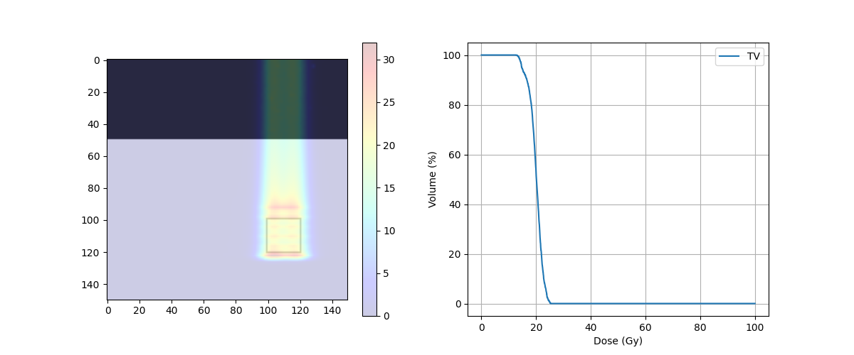
D95 = 18.73779296875 Gy
D5 = 22.6318359375 Gy
D5 - D95 =  3.89404296875 Gy