Bound Constraint Optimization

author: OpenTPS team

In this example, we optimize an ion plan (Protons) using the BoundConstraintsOptimizer function. This function allows optimization with constraints on the Monitor Unit (MU) values of each spot. It helps to stay as close as possible to reality when certain machines cannot accept MU/spot values that are too high or too low.

running time: ~ 15 minutes

Setting up the environment in google collab

import sys
if "google.colab" in sys.modules:
    from IPython import get_ipython
    get_ipython().system('git clone https://gitlab.com/openmcsquare/opentps.git')
    get_ipython().system('pip install ./opentps')
    get_ipython().system('pip install scipy==1.10.1')
    import opentps

imports

import math
import os
import logging
import numpy as np
from matplotlib import pyplot as plt
import sys
sys.path.append('..')

import the needed opentps.core packages

from opentps.core.data.images import CTImage
from opentps.core.data.images import ROIMask
from opentps.core.data.plan import ObjectivesList
from opentps.core.data.plan import ProtonPlanDesign
from opentps.core.data import DVH
from opentps.core.data import Patient
from opentps.core.data.plan import FidObjective
from opentps.core.io import mcsquareIO
from opentps.core.io.scannerReader import readScanner
from opentps.core.io.serializedObjectIO import saveRTPlan, loadRTPlan
from opentps.core.processing.doseCalculation.doseCalculationConfig import DoseCalculationConfig
from opentps.core.processing.doseCalculation.protons.mcsquareDoseCalculator import MCsquareDoseCalculator
from opentps.core.processing.imageProcessing.resampler3D import resampleImage3DOnImage3D, resampleImage3D
from opentps.core.processing.planOptimization.planOptimization import BoundConstraintsOptimizer, IntensityModulationOptimizer
logger = logging.getLogger(__name__)

Output path

We will create an output folder to store the results of this example

output_path = 'Output'
if not os.path.exists(output_path):
    os.makedirs(output_path)
logger.info('Files will be stored in {}'.format(output_path))

Generic CT creation

we will first create a generic CT of a box fill with water and air

ctCalibration = readScanner(DoseCalculationConfig().scannerFolder)
bdl = mcsquareIO.readBDL(DoseCalculationConfig().bdlFile)

patient = Patient()
patient.name = 'Patient'

ctSize = 150

ct = CTImage()
ct.name = 'CT'
ct.patient = patient

huAir = -1024.
huWater = ctCalibration.convertRSP2HU(1.)
data = huAir * np.ones((ctSize, ctSize, ctSize))
data[:, 50:, :] = huWater
ct.imageArray = data

Region of interest

we will now create a region of interest wich is a small 3D box of size 20*20*20

roi = ROIMask()
roi.patient = patient
roi.name = 'TV'
roi.color = (255, 0, 0) # red
data = np.zeros((ctSize, ctSize, ctSize)).astype(bool)
data[100:120, 100:120, 100:120] = True
roi.imageArray = data

Configuration of Mcsquare

To configure the MCsquare calculator we need to calibrate it with the CT calibration obtained above

mc2 = MCsquareDoseCalculator()
mc2.beamModel = bdl
mc2.ctCalibration = ctCalibration
mc2.nbPrimaries = 5e4

Plan Creation

# Design plan
beamNames = ["Beam1"]
gantryAngles = [0.]
couchAngles = [0.]

# Load / Generate new plan
plan_file = os.path.join(output_path,"Plan_WaterPhantom_cropped_resampled.tps")

if os.path.isfile(plan_file):
    plan = loadRTPlan(plan_file)
    logger.info('Plan loaded')
else:
    planInit = ProtonPlanDesign()
    planInit.ct = ct
    planInit.gantryAngles = gantryAngles
    planInit.beamNames = beamNames
    planInit.couchAngles = couchAngles
    planInit.calibration = ctCalibration
    planInit.spotSpacing = 5.0
    planInit.layerSpacing = 5.0
    planInit.targetMargin = 5.0
    planInit.setScoringParameters(scoringSpacing=[2, 2, 2], adapt_gridSize_to_new_spacing=True)
    # needs to be called after scoringGrid settings but prior to spot placement
    planInit.defineTargetMaskAndPrescription(target = roi, targetPrescription = 20.)

    plan = planInit.buildPlan()  # Spot placement
    plan.PlanName = "NewPlan"

    beamlets = mc2.computeBeamlets(ct, plan, roi=[roi])
    plan.planDesign.beamlets = beamlets

    beamlets.storeOnFS(os.path.join(output_path, "BeamletMatrix_" + plan.seriesInstanceUID + ".blm"))

    saveRTPlan(plan, plan_file)

# Set objectives (attribut is already initialized in planDesign object)
plan.planDesign.objectives.addFidObjective(roi, FidObjective.Metrics.DMAX, 20.0, 1.0)
plan.planDesign.objectives.addFidObjective(roi, FidObjective.Metrics.DMIN, 20.5, 1.0)

solver = BoundConstraintsOptimizer(method='Scipy_L-BFGS-B', plan=plan, maxiter=50, bounds=(0.2, 50))

Optimize treatment plan

doseImage, ps = solver.optimize()

Dose volume histogram

target_DVH = DVH(roi, doseImage)
print('D95 = ' + str(target_DVH.D95) + ' Gy')
print('D5 = ' + str(target_DVH.D5) + ' Gy')
print('D5 - D95 =  {} Gy'.format(target_DVH.D5 - target_DVH.D95))

D95 = 18.95751953125 Gy
D5 = 21.35009765625 Gy
D5 - D95 =  2.392578125 Gy

Center of mass

Here we look at the part of the 3D CT image where “stuff is happening” by getting the CoM. We use the function resampleImage3DOnImage3D to the same array size for both images.

roi = resampleImage3DOnImage3D(roi, ct)
COM_coord = roi.centerOfMass
COM_index = roi.getVoxelIndexFromPosition(COM_coord)
Z_coord = COM_index[2]

img_ct = ct.imageArray[:, :, Z_coord].transpose(1, 0)
contourTargetMask = roi.getBinaryContourMask()
img_mask = contourTargetMask.imageArray[:, :, Z_coord].transpose(1, 0)
img_dose = resampleImage3DOnImage3D(doseImage, ct)
img_dose = img_dose.imageArray[:, :, Z_coord].transpose(1, 0)

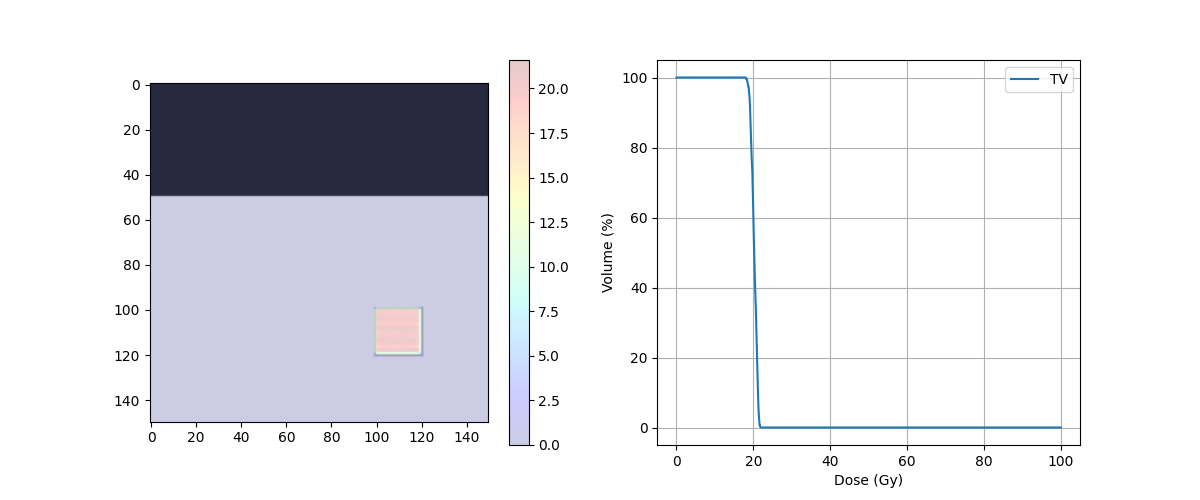
Plot of the dose

fig, ax = plt.subplots(1, 2, figsize=(12, 5))
ax[0].imshow(img_ct, cmap='gray')
ax[0].imshow(img_mask, alpha=.2, cmap='binary')
dose = ax[0].imshow(img_dose, cmap='jet', alpha=.2)
plt.colorbar(dose, ax=ax[0])
ax[1].plot(target_DVH.histogram[0], target_DVH.histogram[1], label=target_DVH.name)
ax[1].set_xlabel("Dose (Gy)")
ax[1].set_ylabel("Volume (%)")
plt.grid(True)
plt.legend()
plt.show()
plt.savefig(f'{output_path}/Dose_BoundContraintOpti.png', format = 'png')
plt.show()