Proton Plan Creation and Dose Calculation

author: OpenTPS team

This example demonstrates how to create a proton plan and perform dose calculation using OpenTPS.

running time: ~ 5 minutes

Setting up the environment in google collab

import sys
if "google.colab" in sys.modules:
    from IPython import get_ipython
    get_ipython().system('git clone https://gitlab.com/openmcsquare/opentps.git')
    get_ipython().system('pip install ./opentps')
    get_ipython().system('pip install scipy==1.10.1')
    import opentps

imports

import os
import logging
import sys

import the needed opentps.core packages

from matplotlib import pyplot as plt

from opentps.core.processing.imageProcessing.resampler3D import resampleImage3DOnImage3D
from opentps.core.processing.planOptimization.tools import evaluateClinical
sys.path.append('..')
import numpy as np

from opentps.core.data.plan import ProtonPlan, RTPlan
from opentps.core.io.scannerReader import readScanner
from opentps.core.io.serializedObjectIO import loadRTPlan, saveRTPlan
from opentps.core.io.dicomIO import readDicomDose, readDicomPlan
from opentps.core.io.dataLoader import readData
from opentps.core.data.CTCalibrations.MCsquareCalibration._mcsquareCTCalibration import MCsquareCTCalibration
from opentps.core.io import mcsquareIO
from opentps.core.data._dvh import DVH
from opentps.core.processing.doseCalculation.doseCalculationConfig import DoseCalculationConfig
from opentps.core.processing.doseCalculation.protons.mcsquareDoseCalculator import MCsquareDoseCalculator
from opentps.core.io.mhdIO import exportImageMHD
from opentps.core.data.plan import PlanProtonBeam
from opentps.core.data.plan import PlanProtonLayer
from opentps.core.data.images import CTImage, DoseImage
from opentps.core.data import RTStruct
from opentps.core.data import Patient
from opentps.core.data.images import ROIMask
from pathlib import Path

logger = logging.getLogger(__name__)

Output path

output_path = os.getcwd()

logger.info('Files will be stored in {}'.format(output_path))

Create plan from scratch and save it

plan = ProtonPlan()
plan.appendBeam(PlanProtonBeam())
plan.appendBeam(PlanProtonBeam())
plan.beams[1].gantryAngle = 120.
plan.beams[0].appendLayer(PlanProtonLayer(100))
plan.beams[0].appendLayer(PlanProtonLayer(90))
plan.beams[1].appendLayer(PlanProtonLayer(80))
plan[0].layers[0].appendSpot([-1,0,1], [1,2,3], [0.1,0.2,0.3])
plan[0].layers[1].appendSpot([0,1], [2,3], [0.2,0.3])
plan[1].layers[0].appendSpot(1, 1, 0.5)

# Save plan
saveRTPlan(plan,os.path.join(output_path,'dummy_plan.tps'))

Load plan in OpenTPS format (serialized)

plan2 = loadRTPlan(os.path.join(output_path,'dummy_plan.tps'))
print(plan2[0].layers[1].spotWeights)
print(plan[0].layers[1].spotWeights)

# Load DICOM plan
#dicomPath = os.path.join(Path(os.getcwd()).parent.absolute(),'opentps','testData','Phantom')
#print(dicomPath)
#dataList = readData(dicomPath, maxDepth=1)
#plan3 = [d for d in dataList if isinstance(d, RTPlan)][0]
# or provide path to RTPlan and read it
# plan_path = os.path.join(Path(os.getcwd()).parent.absolute(),'opentps/testData/Phantom/Plan_SmallWaterPhantom_cropped_resampled_optimized.dcm')
# plan3 = readDicomPlan(plan_path)

[0.2 0.3]
[0.2 0.3]

Dose computation from plan

Choosing default Scanner and BDL

doseCalculator = MCsquareDoseCalculator()
doseCalculator.ctCalibration = readScanner(DoseCalculationConfig().scannerFolder)
doseCalculator.beamModel = mcsquareIO.readBDL(DoseCalculationConfig().bdlFile)
doseCalculator.nbPrimaries = 1e7

Generic example: box of water with spherical target

# Load CT & contours
# ct = [d for d in dataList if isinstance(d, CTImage)][0]
# struct = [d for d in dataList if isinstance(d, RTStruct)][0]
# target = struct.getContourByName('TV')
# body = struct.getContourByName('Body')

# or create CT and contours
ctSize = 20
ct = CTImage()
ct.name = 'CT'

target = ROIMask()
target.name = 'TV'
target.spacing = ct.spacing
target.color = (255, 0, 0)  # red
targetArray = np.zeros((ctSize, ctSize, ctSize)).astype(bool)
radius = 2.5
x0, y0, z0 = (10, 10, 10)
x, y, z = np.mgrid[0:ctSize:1, 0:ctSize:1, 0:ctSize:1]
r = np.sqrt((x - x0) ** 2 + (y - y0) ** 2 + (z - z0) ** 2)
targetArray[r < radius] = True
target.imageArray = targetArray

huAir = -1024.
huWater = doseCalculator.ctCalibration.convertRSP2HU(1.)
ctArray = huAir * np.ones((ctSize, ctSize, ctSize))
ctArray[1:ctSize - 1, 1:ctSize - 1, 1:ctSize - 1] = huWater
ctArray[targetArray>=0.5] = 50
ct.imageArray = ctArray

body = ROIMask()
body.name = 'Body'
body.spacing = ct.spacing
body.color = (0, 0, 255)
bodyArray = np.zeros((ctSize, ctSize, ctSize)).astype(bool)
bodyArray[1:ctSize- 1, 1:ctSize - 1, 1:ctSize - 1] = True
body.imageArray = bodyArray

# MCsquare simulation
doseImage = doseCalculator.computeDose(ct, plan)
# or Load dicom dose
#doseImage = [d for d in dataList if isinstance(d, DoseImage)][0]
# or
#dcm_dose_file = os.path.join(output_path, "Dose_SmallWaterPhantom_resampled_optimized.dcm")
#doseImage = readDicomDose(dcm_dose_file)

# Export dose
#output_path = os.getcwd()
#exportImageMHD(output_path, doseImage)

DVH

dvh = DVH(target, doseImage)
print("D95",dvh._D95)
print("D5",dvh._D5)
print("Dmax",dvh._Dmax)
print("Dmin",dvh._Dmin)

D95 0
D5 0.06103515625
Dmax 0.02890739
Dmin 0.0067956904

Plot dose

target = resampleImage3DOnImage3D(target, ct)
COM_coord = target.centerOfMass
COM_index = target.getVoxelIndexFromPosition(COM_coord)
Z_coord = COM_index[2]

img_ct = ct.imageArray[:, :, Z_coord].transpose(1, 0)
contourTargetMask = target.getBinaryContourMask()
img_mask = contourTargetMask.imageArray[:, :, Z_coord].transpose(1, 0)
img_dose = resampleImage3DOnImage3D(doseImage, ct)
img_dose = img_dose.imageArray[:, :, Z_coord].transpose(1, 0)

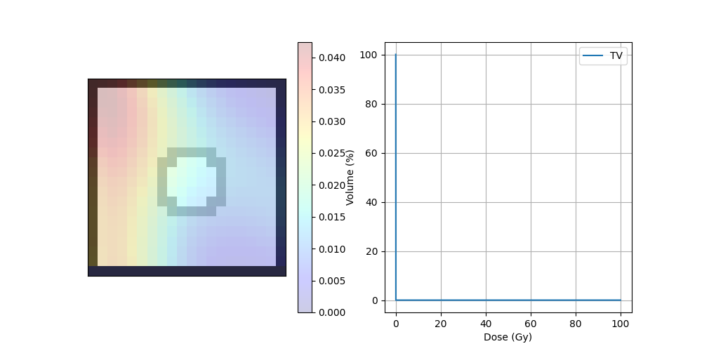
Display dose

fig, ax = plt.subplots(1, 2, figsize=(10, 5))
ax[0].axes.get_xaxis().set_visible(False)
ax[0].axes.get_yaxis().set_visible(False)
ax[0].imshow(img_ct, cmap='gray')
ax[0].imshow(img_mask, alpha=.2, cmap='binary')  # PTV
dose = ax[0].imshow(img_dose, cmap='jet', alpha=.2)
plt.colorbar(dose, ax=ax[0])
ax[1].plot(dvh.histogram[0], dvh.histogram[1], label=dvh.name)
ax[1].set_xlabel("Dose (Gy)")
ax[1].set_ylabel("Volume (%)")
ax[1].grid(True)
ax[1].legend()
plt.show()