Simple dose computation

author: OpenTPS team

In this example we are going to create a generic CT and use the MCsquare dose calculator to compute the dose image

running time: ~ 7 minute

Setting up the environment in google collab

import sys
if "google.colab" in sys.modules:
    from IPython import get_ipython
    get_ipython().system('git clone https://gitlab.com/openmcsquare/opentps.git')
    get_ipython().system('pip install ./opentps')
    get_ipython().system('pip install scipy==1.10.1')
    import opentps

imports

import numpy as np
import os
from matplotlib import pyplot as plt
import math

import the needed opentps.core packages

from opentps.core.data.images import CTImage
from opentps.core.data.images import ROIMask
from opentps.core.data.plan import ProtonPlanDesign
from opentps.core.data import DVH
from opentps.core.data import Patient
from opentps.core.io import mcsquareIO
from opentps.core.io.scannerReader import readScanner
from opentps.core.processing.doseCalculation.doseCalculationConfig import DoseCalculationConfig
from opentps.core.processing.doseCalculation.protons.mcsquareDoseCalculator import MCsquareDoseCalculator
from opentps.core.processing.imageProcessing.resampler3D import resampleImage3DOnImage3D,resampleImage3D

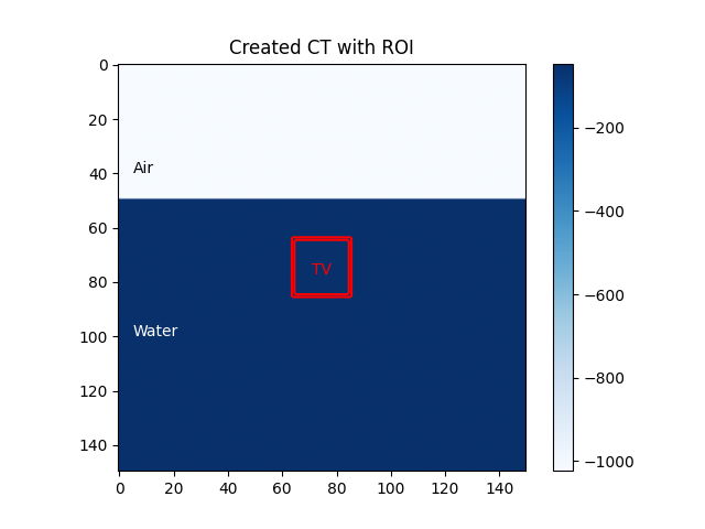
Generic CT creation

we will first create a generic CT of a box fill with water and air

ctCalibration = readScanner(DoseCalculationConfig().scannerFolder)
bdl = mcsquareIO.readBDL(DoseCalculationConfig().bdlFile)

patient = Patient()
patient.name = 'Patient'

ctSize = 150

ct = CTImage()
ct.name = 'CT'
ct.patient = patient

huAir = -1024.
huWater = ctCalibration.convertRSP2HU(1.)
data = huAir * np.ones((ctSize, ctSize, ctSize))
data[:, 50:, :] = huWater
ct.imageArray = data

Region of interest

we will now create a region of interest wich is a small 3D box of size 20*20*20

roi = ROIMask()
roi.patient = patient
roi.name = 'TV'
roi.color = (255, 0, 0) # red
data = np.zeros((ctSize, ctSize, ctSize)).astype(bool)
data[65:85, 65:85, 65:85] = True
roi.imageArray = data

Configuration of MCsquare

to configure Mcsquare we need to calibrate it with the CT calibration obtained above

mc2 = MCsquareDoseCalculator()
mc2.beamModel = bdl
mc2.ctCalibration = ctCalibration
mc2.nbPrimaries = 1e7

Plan Creation

we will now create a plan and create one beam

# Design plan
beamNames = ["Beam1","Beam2","Beam3"]
gantryAngles = [0.,90.,270.]
couchAngles = [0.,0.,0.]

# Generate new plan
planDesign = ProtonPlanDesign()
planDesign.ct = ct
planDesign.targetMask = roi
planDesign.gantryAngles = gantryAngles
planDesign.beamNames = beamNames
planDesign.couchAngles = couchAngles
planDesign.calibration = ctCalibration
planDesign.spotSpacing = 5.0
planDesign.layerSpacing = 5.0
planDesign.targetMargin = 5.0

plan = planDesign.buildPlan()  # Spot placement
plan.PlanName = "NewPlan"

/opt/hostedtoolcache/Python/3.11.13/x64/lib/python3.11/site-packages/opentps/core/processing/planOptimization/planInitializer.py:102: UserWarning: Small proton ranges are used, accuracy of energy computation cannot be guaranteed.
  warnings.warn('Small proton ranges are used, accuracy of energy computation cannot be guaranteed.')

Center of mass

Here we look at the part of the 3D CT image where “stuff is happening” by getting the CoM. We use the function resampleImage3DOnImage3D to the same array size for both images.

roi = resampleImage3DOnImage3D(roi, ct)
COM_coord = roi.centerOfMass
COM_index = roi.getVoxelIndexFromPosition(COM_coord)
Z_coord = COM_index[2]

img_ct = ct.imageArray[:, :, Z_coord].transpose(1, 0)
contourTargetMask = roi.getBinaryContourMask()
img_mask = contourTargetMask.imageArray[:, :, Z_coord].transpose(1, 0)

#Output path
output_path = 'Output'
if not os.path.exists(output_path):
    os.makedirs(output_path)

image = plt.imshow(img_ct,cmap='Blues')
plt.colorbar(image)
plt.contour(img_mask,colors="red")
plt.title("Created CT with ROI")
plt.text(5,40,"Air",color= 'black')
plt.text(5,100,"Water",color = 'white')
plt.text(71,77,"TV",color ='red')
plt.savefig(os.path.join(output_path, 'SimpleCT.png'),format = 'png')
plt.show()

Dose Computation

We now use the MCsquare dose calculator to compute the dose of the created plan

doseImage = mc2.computeDose(ct, plan)

img_dose = resampleImage3DOnImage3D(doseImage, ct)
img_dose = img_dose.imageArray[:, :, Z_coord].transpose(1, 0)
scoringSpacing = [2, 2, 2]
scoringGridSize = [int(math.floor(i / j * k)) for i, j, k in zip([150,150,150], scoringSpacing, [1,1,1])]
roiResampled = resampleImage3D(roi, origin=ct.origin, gridSize=scoringGridSize, spacing=scoringSpacing)
target_DVH = DVH(roiResampled, doseImage)

fig, ax = plt.subplots(1, 2, figsize=(12, 5))
ax[0].imshow(img_ct, cmap='gray')
ax[0].imshow(img_mask, alpha=.2, cmap='binary')  # PTV
dose = ax[0].imshow(img_dose, cmap='jet', alpha=.2)
cbar = plt.colorbar(dose, ax=ax[0])
cbar.set_label('Dose(Gy)')
ax[1].plot(target_DVH.histogram[0], target_DVH.histogram[1], label=target_DVH.name)
ax[1].set_xlabel("Dose (Gy)")
ax[1].set_ylabel("Volume (%)")
plt.grid(True)
plt.legend()
plt.savefig(os.path.join(output_path, 'SimpleDose.png'), format = 'png')
plt.show()

print('D95 = ' + str(target_DVH.D95) + ' Gy')
print('D5 = ' + str(target_DVH.D5) + ' Gy')
print('D5 - D95 =  {} Gy'.format(target_DVH.D5 - target_DVH.D95))

D95 = 10.900181361607142 Gy
D5 = 16.368001302083332 Gy
D5 - D95 =  5.46781994047619 Gy