Photon Plan Creation and Dose Calculation

author: OpenTPS team

This example demonstrates how to create a photon plan and perform dose calculation using OpenTPS.

running time: ~ 10 minutes

Setting up the environment in google collab

import sys
if "google.colab" in sys.modules:
    from IPython import get_ipython
    get_ipython().system('git clone https://gitlab.com/openmcsquare/opentps.git')
    get_ipython().system('pip install ./opentps')
    get_ipython().system('pip install scipy==1.10.1')
    import opentps

imports

import os
from opentps.core.data.images._ctImage import CTImage
from opentps.core.io.scannerReader import readScanner
from opentps.core.processing.doseCalculation.doseCalculationConfig import DoseCalculationConfig
from opentps.core.processing.doseCalculation.photons.cccDoseCalculator import CCCDoseCalculator
from opentps.core.io.sitkIO import exportImageSitk
import numpy as np
from opentps.core.data.images import ROIMask
import logging
from opentps.core.data.plan._photonPlan import PhotonPlan
from opentps.core.data.plan._planPhotonBeam import PlanPhotonBeam
from opentps.core.data.plan._planPhotonSegment import PlanPhotonSegment
from opentps.core.io.serializedObjectIO import loadRTPlan, saveRTPlan
from pathlib import Path
from opentps.core.processing.imageProcessing.resampler3D import resampleImage3DOnImage3D
from opentps.core.data._dvh import DVH
import matplotlib.pyplot as plt

logger = logging.getLogger(__name__)

def getMLCCoordinates(Ymin, Ymax, step):
    first_column = np.arange(Ymin, Ymax, step)
    second_column = np.arange(Ymin + step, Ymax + step, step)
    Xl = np.zeros(len(first_column))
    Xr =  np.zeros(len(first_column))
    # Xl[15:25] = np.random.rand(10) * -5
    # Xr[15:25] = np.random.rand(10) * 5
    Xl[15:25] = np.ones(10) * -5
    Xr[15:25] = np.ones(10) * 5
    return np.column_stack((first_column, second_column, Xl, Xr))

def initializeSegment(beamSegment,Ymin, Ymax, step):
    beamSegment.Xmlc_mm = getMLCCoordinates(Ymin, Ymax, step)
    beamSegment.x_jaw_mm = [-50, 50]
    beamSegment.y_jaw_mm = [-200, 200]
    beamSegment.mu = 5000

Output path

output_path = os.path.join(os.getcwd(), 'Output_Example','PhotonDoseCalculation')
if not os.path.exists(output_path):
    os.makedirs(output_path)

logger.info('Files will be stored in {}'.format(output_path))

Create plan from scratch

plan = PhotonPlan()
plan.appendBeam(PlanPhotonBeam())
plan.appendBeam(PlanPhotonBeam())
plan.beams[0].appendBeamSegment(PlanPhotonSegment())
plan.beams[1].appendBeamSegment(PlanPhotonSegment())

Ymax = 200
Ymin = -200
step = 10
initializeSegment(plan.beams[0].beamSegments[0], Ymin, Ymax, step)
initializeSegment(plan.beams[1].beamSegments[0], Ymin, Ymax, step)
plan.beams[1].beamSegments[0].gantryAngle_degree = 90.

# Save plan
saveRTPlan(plan,os.path.join(output_path,'dummy_plan.tps'))

# Load plan
plan2 = loadRTPlan(os.path.join(output_path,'dummy_plan.tps'))
print(plan2)

Beam
                Beam type: Static
                There are 1 beam segments. In total they have 0 beamlets.
Beam
                Beam type: Static
                There are 1 beam segments. In total they have 0 beamlets.

Dose computation from plan

ccc = CCCDoseCalculator(batchSize= 30)
ccc.ctCalibration = readScanner(DoseCalculationConfig().scannerFolder)

Create CT and contours

ctSize = 20
ct = CTImage()
ct.name = 'CT'
ct.origin = -ctSize/2 * ct.spacing

target = ROIMask()
target.name = 'TV'
target.origin = -ctSize/2 * ct.spacing
target.spacing = ct.spacing
target.color = (255, 0, 0)  # red
targetArray = np.zeros((ctSize, ctSize, ctSize)).astype(bool)
radius = 2.5
x0, y0, z0 = (10, 10, 10)
x, y, z = np.mgrid[0:ctSize:1, 0:ctSize:1, 0:ctSize:1]
r = np.sqrt((x - x0) ** 2 + (y - y0) ** 2 + (z - z0) ** 2)
targetArray[r < radius] = True
target.imageArray = targetArray

ctArray = np.zeros((ctSize, ctSize, ctSize))
ctArray[1:ctSize - 1, 1:ctSize - 1, 1:ctSize - 1] = 1
ctArray[targetArray>=0.5] = 10
ct.imageArray = ctArray

body = ROIMask()
body.name = 'Body'
body.spacing = ct.spacing
body.origin = -ctSize/2 * ct.spacing
body.color = (0, 0, 255)
bodyArray = np.zeros((ctSize, ctSize, ctSize)).astype(bool)
bodyArray[1:ctSize- 1, 1:ctSize - 1, 1:ctSize - 1] = True
body.imageArray = bodyArray

doseImage = ccc.computeDose(ct, plan)

Simplifying plan...
There are 67 beams per batch file

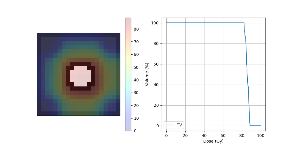
DVH

dvh = DVH(target, doseImage)
print("D95",dvh._D95)
print("D5",dvh._D5)
print("Dmax",dvh._Dmax)
print("Dmin",dvh._Dmin)

D95 82.48291015625
D5 88.22021484375
Dmax 88.52239321754496
Dmin 82.28036653122217

Plot dose

target = resampleImage3DOnImage3D(target, ct)
COM_coord = target.centerOfMass
COM_index = target.getVoxelIndexFromPosition(COM_coord)
Z_coord = COM_index[2]

img_ct = ct.imageArray[:, :, Z_coord].transpose(1, 0)
contourTargetMask = target.getBinaryContourMask()
img_mask = contourTargetMask.imageArray[:, :, Z_coord].transpose(1, 0)
img_dose = resampleImage3DOnImage3D(doseImage, ct)
img_dose = img_dose.imageArray[:, :, Z_coord].transpose(1, 0)

Display dose

fig, ax = plt.subplots(1, 2, figsize=(10, 5))
ax[0].axes.get_xaxis().set_visible(False)
ax[0].axes.get_yaxis().set_visible(False)
ax[0].imshow(img_ct, cmap='gray')
ax[0].imshow(img_mask, alpha=.2, cmap='binary')  # PTV
dose = ax[0].imshow(img_dose, cmap='jet', alpha=.2)
plt.colorbar(dose, ax=ax[0])
ax[1].plot(dvh.histogram[0], dvh.histogram[1], label=dvh.name)
ax[1].set_xlabel("Dose (Gy)")
ax[1].set_ylabel("Volume (%)")
ax[1].grid(True)
ax[1].legend()
plt.savefig(os.path.join(output_path, 'dose.png'))
plt.show()